1. Financial Risks in Capital Projects
Nowadays it seems that an industrial capital investment without risk is not worthy! Actually, the risk-free industrial investment is a non-existing entity, but despite this fact the conventional financial evaluation of projects is still dominated by a static approach. In some cases, a single-point consideration of simple alternative scenarios is included, typically as a sensitivity analysis.
Clearly, not all projects require a risk evaluation, and there are projects which include sophisticated risk analysis in their assessment. But in our opinion most medium to large projects that could benefit from a quantitative risk analysis do not get it, at least in the cement industry.
Why is this?
Perhaps there is no need: maybe projects perform so well that the trouble of conducting a quantitative risk-based approach is not required. Or perhaps such analysis is far too complicated, or the hindsight achieved with it does not justify the effort.
Fact is that overestimation of project financial performance is very common. One sample almost selected at random: “About seven out of ten industrial projects underperform in production, operability, and/or have significant cost or schedule overruns”.[1] But even if it was not and projects delivered as planned, obtaining a better understanding of the expected performance in an uncertain environment can surely provide an advantage to the project owner.
Nowadays it is rather easy to gain a general understanding of the project performance in unchartered waters. A detailed knowledge of the uncertain is indeed difficult, almost by definition, but getting a reasonable estimate of the probabilities around occurrences and consequences is actually not always that complex.
As we will show in this article, the information gained through a rather simple risk evaluation is well worth.
For the purpose of facilitating the exposure we use a real project of the cement industry: we present the standard financial analysis developed at a feasibility study for a decision-gate, and we move forward in the document by adding successive layers of risk evaluation from the finance perspective.
[1] http://www.engineeringnewworld.com/?p=368.
2. The Project
This real case had its construction completed some years ago. It was a brownfield project involving a new kiln line in a Central Asia country. We have modified some of the figures in order to preserve the identification of the works. In brief:
The main contract amounts to 75 USD mio. Design, engineering, and construction take 3 years.
Projects related to the new quarry development and logistics add 18.5 USD mio, also spent in 3 years with 1-year decalage from the main contract. A capex to maintain of 2 USD mio/y is further assumed, although this part was mostly related to the old facilities of the plant.
Production starts with 1.1 Mt/y and reaches 1.5 Mt/y with a 7 years ramp.
Sale prices are increased from 60 USD/t to 80 USD/t in 15 years.
Operational EBIDTA reaches 40% and net income is close to 30% of revenues.
The following table presents the main financial projections in some detail.
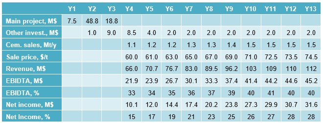
Table 1: Main Financial Projections
For a WACC of 12% the project yields:
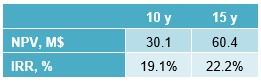
Table 2: Main Financial Results
The cash-flows are presented in the following charts.
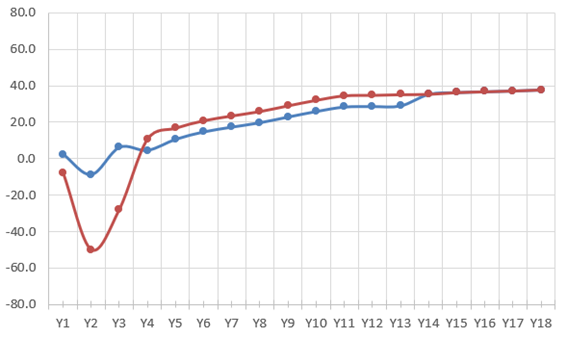
Figure 1: Net Cash-Flows (M$/y; blue: total; burgundy: operations)
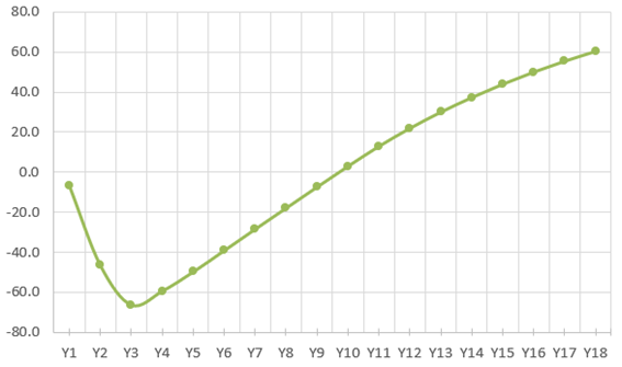
Figure 2: Cumulated Discounted Operational Net Cash-Flows (M$/y)
The financial assessment is often completed with the sensitivities. In this case the following scenarios were developed, with the results shown in the table:
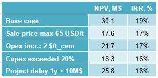
Table 3: Scenarios, Main Financial Results
3. The Case for the Quantitative Risk
The main argument for a quantitative risk assessment is that it can provide much more information about the project behaviour, and this can be achieved not necessarily with complex calculations or arbitrary assumptions.
In the scenarios presented in Table 3: what is special about 65 USD/t or a 20% Capex deviation so that these were the selected thresholds? Actually nothing: they have been selected because the financial analyst had considered that they are good enough representatives of possible conditions that may occur. But no information is provided on the likelihood of these cases, or their combinations. Capex exceedance, Opex increases and sale price capping are, as far as one can judge, independent factors, so why their simultaneous occurrence was not considered? Also, although the purpose of the sensitivity analysis is to verify that a minimum set of financial conditions are met, why the risk of better than expected events is not assessed?
Our point is that a simple quantitative risk analysis that requires little more additional information can yield a significant increase in the insights of the project performance.
Let’s proof it! We’ll start with the scenarios used in the standard financial assessment and develop them one step forward.
3.1 Simulation
We have developed a statistical computer model and run 1,000 simulations.
3.2 Sales Volume
The sensibility scenarios presented in Table 3 did not consider a deviation from the specified sales. This is surprising considering that sales volume is a key direct driver of profitability, and they show a tendency to vagaries. But perhaps this market was somehow special.
In a domestic market, cement sales are affected by share and the overall national consumption. As a starter, it is clearly difficult to make a prediction on the behaviour of a domestic market, but in this case we have the advantage of the hindsight. The following chart presents the cement production and consumption before and after the year-0 in the project’s country.
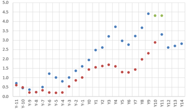
Figure 3: Domestic Market (Mt/y; blue: consumption, burgundy: production)
In the 10 years following the start of production of the new project, the total domestic production was below the assumed scenarios in 3 years.
We are not entering into the details of the country’s cement industry, but it is clear that the scenarios used for the assessment of the project did not adequately forecast the reality. They were wrong, even though it was a particularly protected market.
Combining the market share with the market size increases the forecasting difficulty. What is relevant here is that while a scenario analysis is focused on a point-estimate, a quantitative risk assessment can easily provide a wider view. And it does not need to be highly sophisticated!
The static scenario assumes a well-defined path of the variable through time, often with a simple forecasting formula, linear (constant absolute increase) or exponential (constant rate of increase). There are alternatives to this static approach, as indicated in the following lines.
The simpler alternative is to define a domain from where independent random variables take values. Unless the path itself is critical, this is an easy approach that may yield good enough results.
It is also possible to generate synthetic paths with random behaviour subject to constraints related, for instance, to historical data or forecasts. This approach is probably the most realistic but requires data and involves certain analytical sophistication.
For our case, an intermediate alternative can be rather easily devised as follows:
- The production at first year varies between 1.0 and 1.2 Mt/y (1.1 Mt/y in the “static” case).
The maximum production that is achieved in the assessed period ranges between 1.2 and 1.5 Mt/y, with larger probability towards the higher values (1.5 Mt/y in the “static” case).
The maximum production is achieved between the years 6th and 10th after project completion (8th year in the “static” case).
There is a linear ramp from production start until reaching the maximum production, although its three parameters have been randomized, as described above.
After reaching maximum production, it remains stable within a range of ±5% (0% in the “static” case).
These hypotheses actually do not consider the possibility of a contracting market, as it actually happened, although it can be introduced. But with their simplicity they allow for slow growing scenarios, as well as for better than planned options! The following chart shows this.
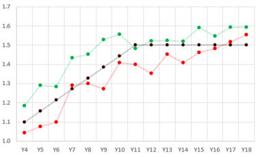
Figure 4: Sales (Mt/y; black: static case; green and red: sample paths above and below the static case)
Overall, this scenario is slightly more conservative than the “static” case, as measured by the average annual growth rate until maximum capacity is reached:
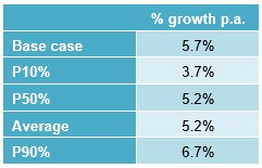
Table 4: Risk Assessment, Production Growth
The following chart and table present the resulting probability distribution of NPV and IRR created by this change in the assumptions.
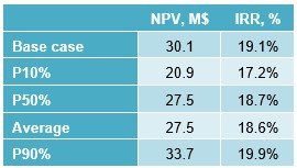
Table 5: Risk Assessment, Production Volume
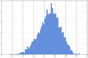
Figure 5: NPV Probability Distribution (M$)
Indeed, a significant modification in perspective from what the static view provided: close to 10% of the expected NPV is, apparently, at risk only because of this change!
3.3 Which Variables to Take into Account?
Sales price, production costs, capex budget, project schedule: all variables affecting the financial analysis can be introduced in the risk model. Of course, it is necessary to remain mindful about the meaning of the risk models and maintain a reasonable borderline in order to avoid the hubris of playing with the powerful tool, whose incorrect utilization just provides a false sense of precision.
For instance: oil prices, currency exchange or the overall condition of the domestic economy can seriously affect almost any project. But the knowledge necessary to properly include them in a risk model as presented in this article is, probably, scarce, so it is often better to treat these risks separately.
The tool described here provides useful means to create and analyse scenarios, but a previous phase of risk identification and classification is necessary.
3.4 Combination of Effects
It is not required to enter into the details, but we have created a model with the following risks and treatment:
Operational costs have a deviation from the “static” case with values drawn from the interval [-1, +2] USD/t.
The core capex budget deviation is within [-5%, +20%].
The project has a delay within [-3, +12] months.
For simplicity we assume there is little relationship between project delay and additional Capex, although the completion delay postpones the start of production and sales.
And the results are:
the NPV will be below the base-case estimate with an estimated probability of 85%,
the same will happen to the IRR,
the most probable NPV and IRR are 23.8 USD mio and 17.6%, resp.
with an estimated probability of 90%, the NPV and IRR will exceed 15.4 USD mio and 15.6%.
A considerable difference, which could had been easily spotted, and which was only irregularly presented by the sensitivity/scenario analysis!
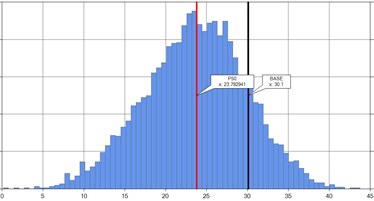
Figure 6: NPV Probability Distribution (M$)
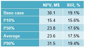
Table 6: Risk Assessment
You can also download the article with this Link